Preface

This research guide consists of two parts. The text part covers the background of the project, introduction and motif-find algorithm analysis. The video part covers the pre-processing method for fMRI of brain regions, ROI selection.

Background

In the study of human intelligence, researchers have long sought to understand the relationship between the functional organization of the brain and individual cognitive abilities. One approach to this problem is to use functional MRI to obtain the brain network in response to a particular stimulus, and then apply algorithms based on graph theory to analyze the structure and function of the network. In this project, two brain network modeling methods were implemented: regularized inverse covariance(Schmidt, 2006) and Conservative PC (CPC) (Ramsey et al, 2006). Three motif-searching methods were also used to analyze changes in network motif over time: FANMOD (Wernicke and Rasche, 2006), MAVisto (Schreiber and Schwöbbermeyer, 2005), and GK (Grochow et al, 2007). These algorithms were applied to data collected from participants performing twelve subtasks from an established intelligence test in order to uncover patterns and temporal information in the brain network. The fMRI dataset under 12 subtasks of this project is from Openneuro (https://openneuro.org/) based on the paper(Soreq et al, 2021). The process of the dataset uses SPM12(https://www.fil.ion.ucl.ac.uk/spm/software/spm12/), Marsbar (https://marsbar-toolbox.github.io/) and AFNI (https://afni.nimh.nih.gov/).

Why I Made This

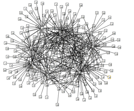
Fig1: Network generated from fMRI data by L1 precision algorithm
I am an undergraduate student majoring in Computer Science at the University of Michigan. I also have a minor in Complex Systems and Statistics. In the fall semester of 2022, I took the class CONMPLXSYS501 Introduction to complex systems. I was fascinated by many of the concepts in complex systems, especially the section on network analysis, especially for its application in neuroscience. Understanding how the human brain works may help us to explore the potential of artificial intelligence and to accomplish real artificial intelligence. Therefore, I chose the analysis of brain networks for my final project.

So, I decided to focus on the analysis of brain networks for my final project, but found the project to be more challenging than I had anticipated. In order to better understand the topic, I spent a considerable amount of time researching neuroscience concepts and learning about the processing of fMRI data and the pros and cons of different algorithms for network modeling. Despite facing limited personal computing resources and other challenges, I persevered and completed my project. This experience has given me a deeper appreciation for the rigors of scientific research and the thrill of exploring uncharted territory.

Introduction

A network motif is a small, recurring pattern that occurs within the structure of a network. These patterns are thought to play a key role in the functioning of the network by providing a basic building block for the organization and operation of the system. For example, in a biological network, a motif might represent a specific interaction between proteins that has a particular biological function. To do this in brain, researchers use functional magnetic resonance imaging (fMRI) data to construct brain networks, and then apply algorithms based on graph theory to search for network motifs. However, motif research on Brain Network focus more on Resting-State network or under single task.
Static data cannot help us understand the underlying logic of how the brain operates. To solve this problem, I modeled brain fMRI for subjects participating in each of the 12 intelligence tests, and perform motif finding algorithm to them. This can help to reveal underlying organizational principles in brain and to understand how these patterns may be related to cognitive processes and behavior.

Approach

The project pipeline consists of the following three parts.

1. pre-processing of FMRI timing data and selection of region of interest (ROI)
2. acquiring the voxel timing signal and obtaining the brain network by network modeling.
3. finding the feature nodes in the network using the motif finding algorithm.
   

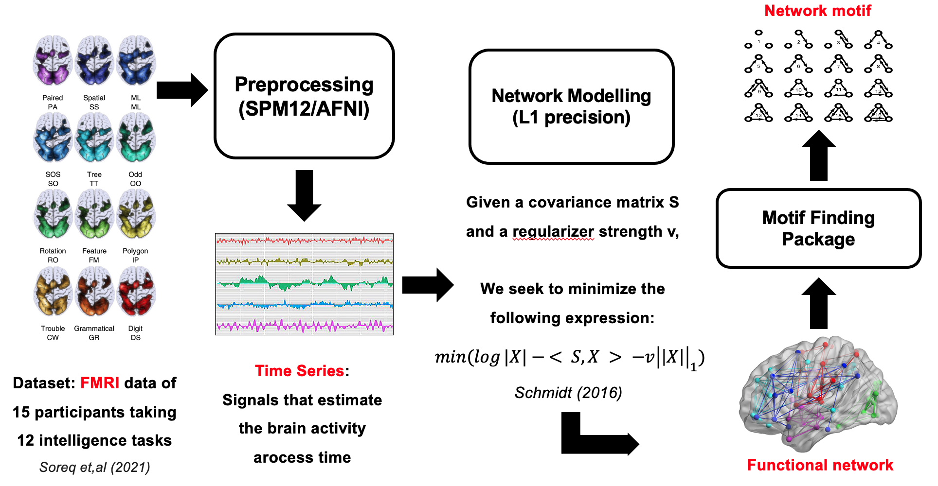
Fig2: pipeline of this project, containing pre-processing, network-modeling and motif-finding

Introduction to Basic Concepts

fMRI Pre-processing & ROI Selection

Network-modeling & Motif Finding

Network-modeling

In this study, the time-series data obtained from the previous step are fed into two algorithms, L1 precision(Schmidt, 2006) and Conservative PC (CPC)(Ramsey et al, 2006), to obtain undirected and directed graphs of brain network connectivity. L1 precision is a method that minimizes the log determinant of the matrix of connectivity weights while constraining the matrix to match the covariance of the input time-series data. This regularization helps to reduce the influence of noise in the data when the number of time points is limited (Smith et al, 2011). CPC is a variant of the PC algorithm that infers causal relationships between the time-series data. It uses a set of rules to determine the orientation of the edges in the network, with the goal of limiting the number of false orientations(Ramsey et al, 2006; Smith et al, 2010). Since L1 precision is effective at identifying direct relationships between the time-series data, while CPC is particularly good at inferring causal relationships. By applying both methods, this study aims to uncover the different topological properties of functional connectivity in the brain.

Motif-finding

Network motif-finding algorithms are a class of computational methods used to identify recurrent patterns of connections within a network. These algorithms can be distinguished into two broad categories: frequency-based and significance-based. Frequency-based algorithms determine the number of occurrences of each motif within a network and report the most frequent motifs. In contrast, significance-based algorithms evaluate whether the observed number of occurrences of each motif is statistically significant compared to a null model of the network. In this study, three motif search algorithms or packages are used to identify network motifs in the brain connectivity data: FANMOD, MAVisto, and Grochow-Kellis.

1. FANMOD (Wernicke and Rasche, 2006) is an efficient algorithm that uses unbiased nodes to sample the network and ensures that each subgraph is only searched once, without generating redundant or meaningless subgraphs. It employs a new analysis method called DIRECT to assess the significance of identified subgraphs, rather than using random networks as null models.
2. MAVisto (Wernicke and Rasche, 2006), on the other hand, uses a pattern tree and the downward closure property to build subnodes by adding edges one by one according to the root nodes. It then evaluates whether the current subgraph is below a predefined threshold and, if so, discards any remaining new or reversed edges until there are none left.
3. The Grochow-Kellis (Grochow et al, 2007) algorithm aims to find all possible mappings of a given query graph in the network, which it does by first calculating the symmetric breaking condition of the query graph and then using the branch and bound method to search for all possible mappings that meet this condition. These three algorithms represent different classes of motif search methods and can be used to evaluate and compare the results of motif searches in the brain connectivity data.

Conclusion

In this study, a total of 15 subjects are selected to undergo motif analysis. For each subject, 12 undirected graphs are inferred from L1 precision and 12 directed graphs are inferred from Conservative PC (CPC) for each of the 12 tasks. Then, for each graph, motif searching is performed using the three algorithms described above to identify motifs with 3, 4, and 5 nodes. The results from all 15 subjects are averaged for each task to obtain the motif distribution for 3, 4, and 5 nodes from both the undirected and directed graphs. This allows for the comparison of the unique motif search results for each task.

After combining the results from the FANMOD, MAVisto, and Grochow-Kellis algorithms, it was found that the dominant motifs identified by these methods are similar. Therefore, the results from FANMOD were used for further analysis.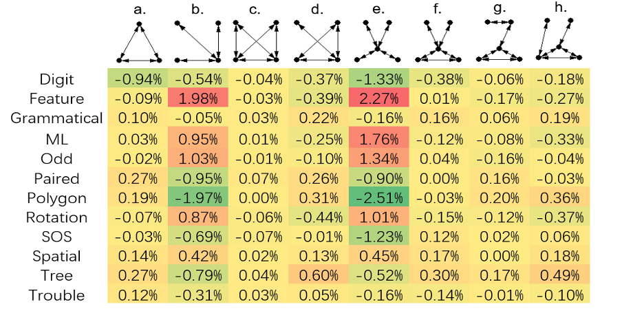

Fig3: The representative motif found in undirected network with 3, 4 or 5 nodes
In the results obtained from the undirected network, only motifs with a p-value <= 0.05 and a frequency >= 0.5% were selected for further analysis. Figure 3 shows the distribution of these motifs for each task, with each row representing a different task and each column representing a different motif. The values in the table are the average frequency of each motif across all tasks, with each value being subtracted from the average to show how far a given motif is from the average value across all tasks.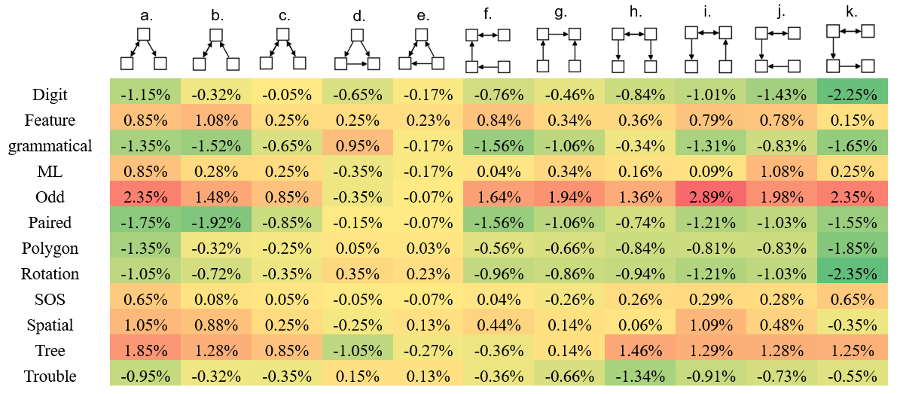

Fig4: The representative motif found in directed network with 3, 4 or 5 nodes
The directed network in Figure 4 exhibits a similar pattern to the undirected network in Figure 3, where different tasks have a distinctive distribution of motifs compared to Figure 3. Motifs that are more responsive to changes in tasks tend to have a high correlation with each other. For example, as shown in Figure 5, Figure 4a and Figure 4j show a correlation value of 0.97, indicating that certain motifs can perform similar functions, even if they are not subnetworks of each other (such as Figure 4a and Figure 4b). Additionally, Figure 4c, Figure 4d, and Figure 4e match motifs found in existing research on brain networks, but show little change among different tasks, possibly indicating that these motifs serve more general functions than others.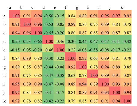

Fig5: The pairwise correlation among a-k
The analysis of the 5-node motifs in the directed network yielded noteworthy results, as several motifs were found to be statistically significant across the 12 tasks studied. However, it was observed that the frequency of the motif AT8NOLYF was disproportionately high in the Digit, Paired, and Polygon tasks, in comparison to both other motifs within these tasks and across other tasks. This suggests that the motif AT8NOLYF may perform a common function among these tasks, as outlined in Alon’s (2007) review of similar motifs.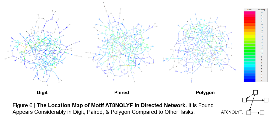

Reference

• Alon, U. (2007). Network motifs: theory and experimental approaches. Nature Reviews Genetics, 8(6), 450-461.
• Grochow, J. A., & Kellis, M. (2007, April). Network motif discovery using subgraph enumeration and symmetry-breaking. In Annual International Conference on Research in Computational Molecular Biology (pp. 92-106). Springer, Berlin, Heidelberg.
• Ramsey, J. Zhang, J. Spirtes, P. (2006). Adjacency-faithfulness and conservative causal inference. Proceedings of the 22nd Annual Conference on Uncertainty in Artificial Intelligence.
• Schmidt, M. (2006) L1precision: Matlab code for MAP estimation of Gaussian Graphical Model Precision with L1-regularizer. Retrieved from http://www.cs.ubc.ca/~schmidtm/Software/L1precision.html.
• Schreiber, F., & Schwöbbermeyer, H. (2005). MAVisto: a tool for the exploration of network motifs. Bioinformatics, 21(17), 3572-3574.
• Soreq, E., Violante, I. R., Daws, R. E., & Hampshire, A. (2021). Neuroimaging evidence for a network sampling theory of individual differences in human intelligence test performance. Nature communications, 12(1), 1-13.
• Wernicke, S., & Rasche, F. (2006). FANMOD: a tool for fast network motif detection. Bioinformatics, 22(9), 1152-1153.

Appendix

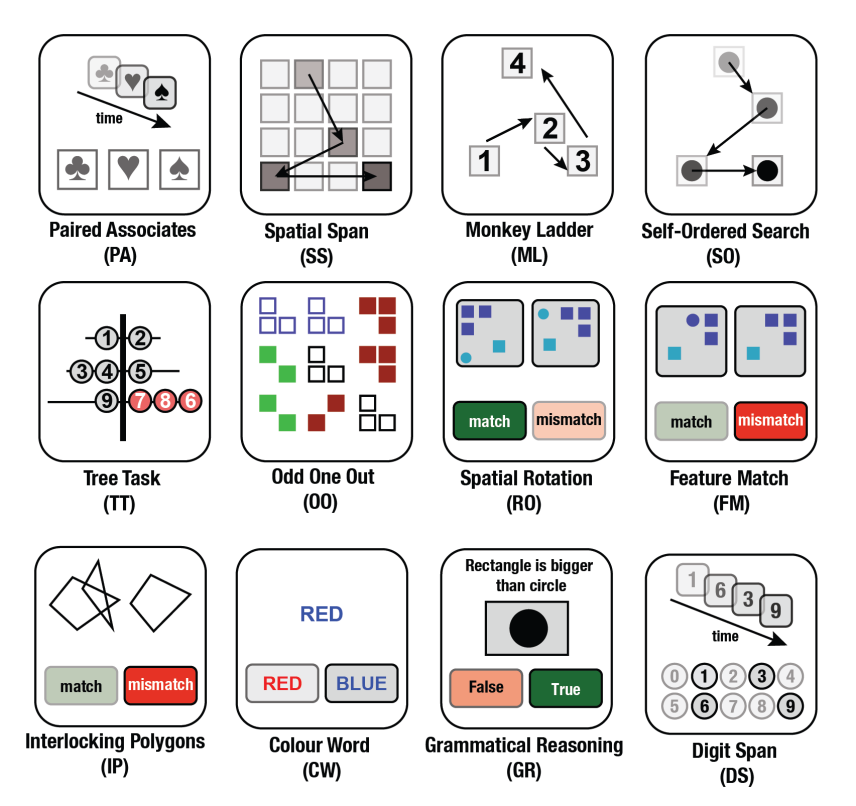
a. Task description
Note: the below information is from supplementary materials of Soreq et al (2021).

1. Paired (PA): This task is based on a paradigm commonly used to assess memory impairments in ageing clinical populations.
2. Spatial (SS): Based on the Corsi Block Tapping Task, which is a classical task for measuring spatial short-term memory capacity.
3. ML (ML): Visuospatial working memory task based on the non-human primate literature.
4. SOS (SO): Based on a test used to measure strategy during search behaviour.
5. Tree (TT): Spatial planning task based on the Tower of London Task, which is widely used to measure executive function.
6. Odd (OO): A deductive reasoning task based on a sub-set of problems from the Cattell Culture Fair Intelligence Test.
7. Rotation (RO): Tasks of this type are typically used to measure the ability to manipulate objects in mind.
8. Feature (FM): Based on classic feature search tasks that have been historically used to measure attentional processing.
9. Polygon (IP): Based on the Interlocking Pentagons task, which is often used in the assessment of age-related disorders.
10. Trouble (CW): (Colour Word) - This is a more challenging variant on the Stroop test.
11. Grammatical (GR): This is a verbal reasoning task based on Alan Baddeley’s 3-minute grammatical reasoning test.
12. Digit (DS): Is a computerised variant on the verbal working memory component of the WAIS-R intelligence test.
    

7 月 21 日 每日一题

17. Letter Combinations of a Phone Number

Given a string containing digits from 2-9 inclusive, return all possible letter combinations that the number could represent. Return the answer in any order.

A mapping of digits to letters (just like on the telephone buttons) is given below. Note that 1 does not map to any letters.

1
2

Input: digits = "23"
Output: ["ad","ae","af","bd","be","bf","cd","ce","cf"]

思路

Using bsf (a queue) or a temp vector to store the intermediate status of the combinations.

代码

1
2
3
4
5
6
7
8
9
10
11
12
13
14
15
16
17
18
19
20
21
22
23

class Solution {
public:
    vector<string> letterCombinations(string digits) {
        if(digits.empty())
            return {};
        vector<string> phone = {"0", "1", "abc", "def", "ghi", "jkl", "mno", "pqrs", "tuv", "wxyz"};
        queue<string> bsf;
        vector<string> ans;
        bsf.push("");
        while(!bsf.empty()){
            string s = bsf.front();
            bsf.pop();
            if(s.length() == digits.length())
                ans.push_back(s);
            else{
                for(char c: phone[digits[s.length()] - '0'])
                    bsf.push(s + c);
            }
        }
        return ans;
    }

};

7 月 20 日 每日一题

543. Diameter of Binary Tree

Given the root of a binary tree, return the length of the diameter of the tree.

The diameter of a binary tree is the length of the longest path between any two nodes in a tree. This path may or may not pass through the root.

The length of a path between two nodes is represented by the number of edges between them.

1
2
3

Input: root = [1,2,3,4,5]
Output: 3
Explanation: 3 is the length of the path [4,2,1,3] or [5,2,1,3].

思路

It is similar to height of tree. Diameter = Height of the left subtree + Height of the right subtree. Keep track of the maxDiameter during traversal by an extra parameter and get the height of the tree.

代码

1
2
3
4
5
6
7
8
9
10
11
12
13
14
15
16
17
18
19
20
21
22
23
24
25
26
27

/**
 * Definition for a binary tree node.
 * struct TreeNode {
 *     int val;
 *     TreeNode *left;
 *     TreeNode *right;
 *     TreeNode() : val(0), left(nullptr), right(nullptr) {}
 *     TreeNode(int x) : val(x), left(nullptr), right(nullptr) {}
 *     TreeNode(int x, TreeNode *left, TreeNode *right) : val(x), left(left), right(right) {}
 * };
 */
class Solution {
public:
    int diameterOfBinaryTree(TreeNode* root) {
        int diameter = 0;
        diaHelper(root, diameter);
        return diameter;
    }
    int diaHelper(TreeNode* node, int& diameter){
        if(!node)
            return 0;
        int left = diaHelper(node->left, diameter);
        int right = diaHelper(node->right, diameter);
        diameter = max(diameter, left + right);
        return max(left,right) + 1;
    }
};

7 月 19 日 每日一题

117. Populating Next Right Pointers in Each Node II

Given a binary tree

struct Node {
int val;
Node *left;
Node *right;
Node *next;
}
Populate each next pointer to point to its next right node. If there is no next right node, the next pointer should be set to NULL.

Initially, all next pointers are set to NULL.

1
2
3

Input: root = [1,2,3,4,5,null,7]
Output: [1,#,2,3,#,4,5,7,#]
Explanation: Given the above binary tree (Figure A), your function should populate each next pointer to point to its next right node, just like in Figure B. The serialized output is in level order as connected by the next pointers, with '#' signifying the end of each level.

思路

The difference between 116 and 117 is that 117 is not a perfect binary tree, which means it cannot be simply solved by recursive.

The direct way is to use iterative BSF. Note that when reach to null, it’s time to move to the next level and add a nullptr to the end of the queue(for the next level end).

There is a O(1) space complexity way, which is a bit similar to double pointer. The detail is in comments of code. Note the when proceed the current level(currParent), the next has been proceed by last while loop.

代码

Way 1:

1
2
3
4
5
6
7
8
9
10
11
12
13
14
15
16
17
18
19
20
21
22
23
24
25
26
27
28
29
30
31
32
33
34
35
36
37
38
39
40
41

/*
// Definition for a Node.
class Node {
public:
    int val;
    Node* left;
    Node* right;
    Node* next;

    Node() : val(0), left(NULL), right(NULL), next(NULL) {}

    Node(int _val) : val(_val), left(NULL), right(NULL), next(NULL) {}

    Node(int _val, Node* _left, Node* _right, Node* _next)
        : val(_val), left(_left), right(_right), next(_next) {}
};
*/
class Solution {
public:
    Node* connect(Node* root) {
        if(root == nullptr)
            return nullptr;
        queue<Node*>q;
        q.push(root);
        q.push(nullptr);
        while(q.size() > 1){
            Node* curr = q.front();
            q.pop();
            if(!curr){
                q.push(nullptr);
                continue;
            }
            curr->next = q.front();
            if(curr->left)
                q.push(curr->left);
            if(curr->right)
                q.push(curr->right);
        }
        return root;
    }
};

Way 2:

1
2
3
4
5
6
7
8
9
10
11
12
13
14
15
16
17
18
19
20
21
22
23
24
25
26
27
28
29
30
31
32
33
34
35
36
37
38
39
40
41
42
43
44

class Solution {
public:
    Node* connect(Node* root) {
        Node *currParent = root;
        Node *baseChild;
        Node *currChild;
        Node *nextChild;
        while(currParent){
            //reach to a parent with at least one child
            while(currParent->next && !currParent->left && !currParent->right)
                currParent = currParent->next;
            //set baseChild and currChild to the first child of the next level
            currChild = baseChild = currParent->left ? currParent->left : currParent->right;
            while(currChild){
                //if currChild is left child and have right sibling
                if(currParent->right && currParent->right != currChild){
                    nextChild = currParent->right;
                }
                else{
                    //move to the adjacent parent
                    currParent = currParent->next;
                    while(currParent && !currParent->left && !currParent->right){
                        currParent = currParent->next;
                        //now currParent has pointed to the next Parent
                    }
                    //if not reach to the end
                    if(currParent){
                        nextChild = currParent->left ? currParent->left : currParent->right;
                    }
                    //if reach to the end
                    else{
                        //if reach to the end of this level
                        nextChild = nullptr;
                    }
                }
                currChild->next = nextChild;
                currChild = nextChild;
            }
            //move to the next level
            currParent = baseChild;
        }
        return root;
    }
};

7 月 18 日 每日一题

时隔两个月的更新，之后会恢复每日一题，频率定为每周六题

116. Populating Next Right Pointers in Each Node

You are given a perfect binary tree where all leaves are on the same level, and every parent has two children. The binary tree has the following definition:

struct Node {
int val;
Node *left;
Node *right;
Node *next;
}
Populate each next pointer to point to its next right node. If there is no next right node, the next pointer should be set to NULL.

Initially, all next pointers are set to NULL.

1
2
3

Input: root = [1,2,3,4,5,6,7]
Output: [1,#,2,3,#,4,5,6,7,#]
Explanation: Given the above perfect binary tree (Figure A), your function should populate each next pointer to point to its next right node, just like in Figure B. The serialized output is in level order as connected by the next pointers, with '#' signifying the end of each level.

思路

For recursive, firstly, point root->left->next to root->right->next. Then use root’s next arrow to find right children’s buddy in the neighboring tree. Take care of current level’s children’s next problem and then move down to children subtree.

代码

1
2
3
4
5
6
7
8
9
10
11
12
13
14
15
16
17
18
19
20
21
22
23
24
25
26
27
28
29
30
31

class Node {
public:
    int val;
    Node* left;
    Node* right;
    Node* next;

    Node() : val(0), left(NULL), right(NULL), next(NULL) {}

    Node(int _val) : val(_val), left(NULL), right(NULL), next(NULL) {}

    Node(int _val, Node* _left, Node* _right, Node* _next)
        : val(_val), left(_left), right(_right), next(_next) {}
};
class Solution {
public:
    Node* connect(Node* root) {
        if(root == nullptr)
            return nullptr;
        if(root->left){
            root->left->next = root->right;
            if(root->next){
                root->right->next = root->next->left;
            }
        }
        connect(root->left);
        connect(root->right);
        return root;
    }

};

Meadow Picnic_2

久违的更新，新开辟的一个 tag，记录现在和以后的摄影作品（可能还算不上作品

5 月 14 日 每日一题

105. Construct Binary Tree from Preorder and Inorder Traversal

One way to serialize a binary tree is to use preorder traversal. When we encounter a non-null node, we record the node’s value. If it is a null node, we record using a sentinel value such as ‘#’.

For example, the above binary tree can be serialized to the string “9,3,4,#,#,1,#,#,2,#,6,#,#”, where ‘#’ represents a null node.

Given a string of comma-separated values preorder, return true if it is a correct preorder traversal serialization of a binary tree.

It is guaranteed that each comma-separated value in the string must be either an integer or a character ‘#’ representing null pointer.

You may assume that the input format is always valid.

For example, it could never contain two consecutive commas, such as “1,,3”.
Note: You are not allowed to reconstruct the tree.

1
2
3
4
5
6
7
8
9
10
11
12

Example 1:

Input: preorder = "9,3,4,#,#,1,#,#,2,#,6,#,#"
Output: true
Example 2:

Input: preorder = "1,#"
Output: false
Example 3:

Input: preorder = "9,#,#,1"
Output: false

思路

本题有两种写法，我用了最笨的一种，每遇到两个#，将这两个 hash 和对应的 leaf node 删掉，然后添加一个#，要注意的是需要使用 while 循环，因为可能会在添加#之后形成新的满足 pop 要求的组合。要注意的是不能直接用 index 访问，因为可能会出现两位数字（92）。
另一种写法是聪明很多，因为 external node 数量必然比 internal 多 1，每遇到一个 val，counter++，遇到#，counter–，如果读完所有的 node 时，count 为-1，则有效（如果未读完所有 node，count 就为 1，意味着此时已经无法插入 node，则此 tree 无效）。

代码

1
2
3
4
5
6
7
8
9
10
11
12
13
14
15
16
17
18
19
20
21
22
23
24
25
26
27
28
29
30
31
32
33
34
35
36
37
38
39
40
41
42
43
44
45
46
47
48
49
50

/**
 * Definition for a binary tree node.
 * struct TreeNode {
 *     int val;
 *     TreeNode *left;
 *     TreeNode *right;
 *     TreeNode() : val(0), left(nullptr), right(nullptr) {}
 *     TreeNode(int x) : val(x), left(nullptr), right(nullptr) {}
 *     TreeNode(int x, TreeNode *left, TreeNode *right) : val(x), left(left), right(right) {}
 * };
 */
class Solution {
public:
    bool isValidSerialization(string preorder) {
        //if it's #
        if(preorder[0] == '#' && preorder.size() == 1)
            return  true;
        else if(preorder[0] == '#' && preorder.size() != 1)
            return false;
        preorder += ',';
        stringstream str(preorder);
        string ele;
        getline(str, ele, ',');
        vector<string> stack;
        stack.push_back(ele);
        while(getline(str, ele, ',')){
            stack.push_back(ele);
            if(stack.back() == "#"){
                while(stack.size() > 2 && stack.back() == "#" && stack[stack.size() - 2] == "#" && stack[stack.size() - 3] != "#" ){
                    stack.pop_back();
                    stack.pop_back();
                    stack.pop_back();
                    stack.push_back("#");
                    }
                }
        }
        if(stack.size() == 1 && stack.back() == "#")
            return true;
        return false;
    }
};

bool isValidSerialization(string p)
{
    stringstream ss{p};
	int c{0};
	for( ; c!=-1 and !ss.eof(); getline(ss, p, ','))
        p[0]=='#' ? --c : ++c；
	return c==-1 and ss.eof();
}